This article is simply me making notes. All credit goes to the authors of the paper.

Introduction

Proteins are one-dimensional polymers of
amino acids ("sequences") that fold into three-dimensional shapes ("structures")

Polymer - large molecule made up of many repeating smaller monomers. In the case of proteins, they are biological polymers made from amino acid monomers. DNA/RNA: monomer = nucleotides.

Proteins have four levels of structure:

• Primary structure: linear sequence of amino acids, order in which amino acids are connected in the chain. Just the order. Determined by the gene’s DNA sequence.

• Secondary structure: local folding patterns that form the H bonds between backbone atoms. Main types are alpha helix, beta sheet and loops/turns/coils. When diffusion models create a backbone, they are implicitly creating secondary structures. The local geometry (bond angles, frame orientations) are different for different types of structures.

• Tertiary structure: Complete 3D fold of a single protein chain and how the entire polypeptide arranges in 3D space. This is what the diffusion models generate.

• Quaternary structure: Multiple protein chains coming together. This applies only if the proteins has multiple chains for example, like Hemoglobin which has 4 separate chains that assemble together. Not all proteins have this structure as many are just one chain.

A residue is a single amino acid unit within a protein chain. So, why is it called a “residue” and not “amino acid”? When amino acids link together to form a protein via a peptide bond, they undergo a condensation reaction that releases a water molecule and what remains after the reaction is the residue. When two amino acids join via a peptide bond, the carboxyl group (-COOH) of one amino acid reacts with the amino group (-NH2) of the next, releasing H2O. Each amino acid in the chain loses some atoms (H and OH), so we call it a residue rather than a complete amino acid. Each residue has backbone atoms: N, Cα (alpha carbon), C and O (same for all residues). Side chain (R group) is unique to each of the 20 amino acid types.

Most generative protein models are sequence-based or structure-based. Sequence-based methods give sequences that ultimately become biomolecules whereas structures require additional structure-to-sequence map (inverse folding). example of sequence model - EvoDiff - discrete diffusion model, uses ByteNet-style architecture for denoising. Structure-based design = prevalent method.

Structure-based methods - model structure space and employ inverse folding models like ProteinMPNN to propose sequences from the generated structure. Structure more closely associates with protein function than sequence.

Genie performs diffusion on backbone atom coordinates and uses an SE(3)-equivariant denoiser to reason over a cloud of reference frames constructed from backbone coordinates

Protein backbone is a set of 3D points (atoms like N, Cα, C, O) in space. In diffusion models, we start with noise and repeatedly denoise to get a realistic sample. Here the thing being noised/denoised is the 3D coordinates of backbone atoms and not pixels. This is similar to RFdiffusion’s approach.

SE(3)-equivariant denoiser: an architectural choice. SE(3) refers to “Special Euclidean group in 3D”. “Special” means the transformations which have determinant +1, excludes reflections, inversions. “Special” transformations preserve orientation(handedness). It refers to the group of all rigid body transformations (rotations + translations). SE(3) equivariance means if you rotate/translate the entire input protein structure, the network’s output rotates/translates in exactly the same way. This is important because proteins don’t have an absolute orientation in space, it is the same protein whether you rotate it 45° or translate it 5 Angstroms. An equivariant network respects this physical symmetry which

• makes the model more data-efficient (since the network does not need to learn the same structure in every possible orientation)

• guarantees physically meaningful outputs

• improves generalization (on data different from training set)

Instead of treating the proteins as a bunch of points, Genie builds local coordinate systems (a “reference frame”) from the backbone at many positions (often per residue). A reference frame is like a local compass with an origin and a rotation comprised of 3 perpendicular axes. Usually, Cα is the origin and axes is defined by directions like Cα→N and Cα→C etc. A “cloud of reference frames” means there are many local frames across the backbone and the model reasons about how these frames relate (distances + relative orientations). With a 100 residues, there will be a 100 local reference frames. Each frame describes the local geometry and orientation at that position in the chain. This is useful because protein structure is about where residues are (translation) and how they are oriented (rotation).

Putting it together:

• Genie starts with noisy backbone coordinates

• converts them into local frames 1 per residue/backbone position

• uses an SE(3) equivariant network to predict how to move/rotate things to denoise

• repeats until a realistic backbone is achieved

Other structure-based models:

• FrameDiff - diffusion process in SE(3) on backbone frames with AlphaFold-inspired architecture for denoising

• FrameFlow - general architecture of FrameDiff but with flow matching

• Chroma - correlated diffusion that accounts for statistical properties of natural proteins with a GNN. Instead of diffusing each atom/residue independently, chroma diffuses in a way that maintains correlations such that nearby residues move together in coordinated ways. The diffusion process is designed so that at each step of denoising, the structure follow the same statistical distributions as real proteins (things like bond angles and distances etc.). Rather than just diffusing arbitrary 3D coordinates, it biases toward protein-like geometries. It also includes a separate design network that predicts sequences and side-chain atoms given a generated backbone.

• Proteus - similar diffusion process and architecture as FrameDiff but uses graph triangle blocks that combine the expressiveness of triangle attention from AlphaFold 2 with faster runtimes by limiting attention to nearby residues.

Structure-based models only generate the geometry - specifically the 3D coordinates of the backbone atoms (N, Cα, C, O) for each residue position. At this stage, it is not decided which amino acid goes at each position, all we know is that there is a residue here at this location with this orientation. So, it is a two-step pipeline that begins with structure generation to generate the backbone coordinates and then inverse folding using models like ProteinMPNN so that given the backbone, we can predict which amino acid sequence would fold into that structure.

Sequence and structure are deeply interconnected. Certain sequences prefer certain structures. If designed separately, you might generate a backbone that’s hard to find a good sequence for or the sequence suggested by ProteinMPNN might not fold stably into the predicted backbone. Integrated approaches:

• RFDiffusion - integrates sequence information as a condition of a structure-based diffusion process

• MultiFlow - performs diffusion/flow matching in a joint sequence-structure space, it combines SE(3) structural flow with a discrete sequence flow.

function is what is sought in protein design

Function in the context of proteins means what the protein does - its biological role or activity. examples:

• Enzymes - DNA polymerase: copies DNA

• Binding function - Hemoglobin: binds and transports oxygen

• Structural function - Collagen: provides mechanical strength to tissues

The goal isn’t to make any protein, we want to make a protein that does something useful.

Most protein functions don’t require the entire protein. They come from small critical regions called motifs. examples:

• Enzyme active site - maybe 5-10 residues that bind and catalyze a substrate (molecule that binds to an enzyme)

• Antibody binding site - small patch that recognizes an antigen

Motif scaffolding is the problem of designing a protein that contains one specific functional motif. So, given a specific motif, existing diffusion models can keep the motif exactly where we want it to be and generate the rest of the protein (remaining residues) around it to form a stable and foldable protein. Models:

• FrameDiff + Twisted Diffusion Sampler (sequential Monte Carlo sampler)

• RFDiffusion

• Updated FrameFlow

But these models cannot design proteins with multiple independent motifs (two or more functional sites that don’t have a fixed known relationship beforehand) unless inter-motif distance and orientation are specified beforehand. But this information is often unknown. Multi-motif is important because many real proteins often have multiple sites, for example multi-substrate enzymes. Hence, this is the motivation to work on multi-motif scaffolding that Genie 2 can do!

Previous Genie Model

Other SE(3)-equivariant diffusion models for protein generations use unified representations for the forward and backward diffusion processes.

Genie represents proteins as point clouds of Cα atoms in the forward process and as clouds of reference frames in the reverse process.

A point cloud is simply a collection of points in 3D space where each point has (x,y,z) coordinates. A point cloud alone doesn’t tell which way each residue is facing nor the local geometry. So, in the reverse process, each residue gets a reference frame (position + orientation) and this way the model reasons about relative positions and rotations not just the distances.

Let $x = [x^1, x^2, ..., x^N]$ be a sequence of Cα coordinates of length N. Given a sample $x_0$ from the unknown protein structure distribution, Genie’s forward process gradually adds isotropic Gaussian noise through a cosine variance schedule $\beta = [\beta_1, \beta_2, ..., \beta_T]$, where T is the total number of diffusion steps (set to 1,000).
$q(x_t|x_{t-1}) = N(x_t|\sqrt{1-\beta_t}x_{t-1}, \beta_tI)$
By reparameterization, we have:
$q(x_t|x_0) = N(x_t|\sqrt{\bar\alpha_t}x_0,(1-\bar\alpha_t)I)$
where $\bar\alpha_t = \prod_{s=1}^{t}\alpha_s$ and $\alpha_t = 1 - \beta_t$.

Isotropic = “same in all directions”. So, isotropic Gaussian noise means the noise is same in all directions = noise has the same variance in every direction (x, y and z). The opposite term is anisotropic. It’s important for the noise to be isotropic for proteins because there is no preferred direction in 3D space for proteins as they don’t care about absolute x, y or z coordinates.

In the forward diffusion process, we want to gradually add noise to a protein structure $x_0$ until it becomes pure Gaussian noise $x_T$. The design goals are:

• Gradual noising - Small steps not sudden jumps

• End at pure noise - After T steps, $x_T$ should be $N(0, I)$

• Markovian - Each step only depends on the previous step

• Simple - Use Gaussian noise since the math is tractable

The general form for the forward process is $x_t = \sqrt{1-\beta_t}x_{t-1} + \sqrt{\beta_t}\epsilon$ where $\epsilon \sim N(0, I)$.

Important things to know:

1. $\epsilon$ is Gaussian and independent of $x_{t-1}$ because $\epsilon$ is freshly sampled noise at each step and hence does not depend on what $x_{t-1}$ is.

2. $x_{t-1}$ is not necessarily Gaussian since it depends on where we are in the process. At t=0, $x_0$ is a real protein structure from the complex distribution of real protein structures. At t=1, $x_1 = \sqrt{1-\beta_1}x_{0} + \sqrt{\beta_1}\epsilon$ which is a mixture of partly real structure (non-Gaussian) and partly noise (Gaussian). As t increases, the distribution of $x_t$ gradually becomes more Gaussian because the signal from $x_0$ gets weaker $(\sqrt{\bar\alpha_t} \to 0)$ and noise accumulates. At t=T(end), $x_T \approx \epsilon \sim N(0, I)$ so now $x_T$ is approximately Gaussian.

3. The conditional distribution $q(x_t|x_{t-1}) = N(x_t|\sqrt{1-\beta_t}x_{t-1}, \beta_tI)$ is Gaussian because we define it that way - Given some specific $x_{t-1}$ (whatever that may be), $x_t$ is Gaussian with that mean and variance.

4. For any random variables $X$ and $Y$, $Var(X + Y) = Var(X) + Var(Y) + 2Cov(X, Y)$ and if they are independent, then $Cov(X, Y) = 0$ so, $Var(X + Y) = Var(X) + Var(Y)$. This is distribution-agnostic.

5. $Var(kX) = k^2Var(X)$

6. We can normalize/center the protein coordinates because of SE(3) geometry. So, we normalize the data to unit variance. Scaling changes the units but not the shape which is all that matters for protein structure. However, once model generates a structure, we need to scale back to physical units because bond lengths have actual physical constraints.

Why this specific form?

1. Why is $\sqrt{1-\beta_t}$ the scaling factor?

   We want to preserve the scale (variance) of the data as we add noise. If we just added noise without scaling: $x_t = x_{t-1} + \sqrt{\beta_t}\epsilon$, the variance would grow unboundedly. Suppose the starting variance is $Var(x_{t-1})$. So now the variance of $x_t = Var(x_t) = Var(\sqrt{1-\beta_t}x_{t-1} + \sqrt{\beta_t}\epsilon = Var(\sqrt{1-\beta_t}x_{t-1}) + Var(\sqrt{\beta_t}\epsilon)$ (We can do this since they are independent) $= (1-\beta_t)Var(x_{t-1}) + \beta_t\cdot1$.

   So, if we want $Var(x_{t-1}) = Var(x_{t})$, we need $(1-\beta_t)Var(x_{t-1}) + \beta_t = Var(x_{t-1})$ which is possible when $Var(x_{t-1}) = 1$, which is achieved by normalizing the data.

2. Why $\beta_t$ and not just $\beta$?

   We use a schedule $\beta_t$ that changes with time:

   • Small $\beta_t$ early on (slow noising, preserve structure)
   • Larger $\beta_t$ later (faster noising as structure is already degraded)

3. Why $\sqrt{\beta_t}$ and not $\beta_t$ for the noise term?

   Because we care about the variance and not standard deviation. We need the noise term to have variance $\beta_t$.

   $Var(\sqrt{\beta_t}\epsilon) = \beta_t \cdot Var(\epsilon) = \beta_t \cdot 1 = \beta_t$

   So, the noise has variance $\beta_t$.

4. Given $x_t = \sqrt{1-\beta_t}x_{t-1} + \sqrt{\beta_t}\epsilon$ for a fixed $x_{t-1}$ and $\epsilon$(we are treating $x_{t-1}$ as a known, fixed value and not a random variable), the mean is:

   $E[x_{t}|x_{t-1}] = E[\sqrt{1-\beta_t}x_{t-1} + \sqrt{\beta_t}\epsilon | x_{t-1}]$

   Since $x_{t-1}$ is fixed, $E[x_{t-1}|x_{t-1}] = x_{t-1}$

   By definition, $\epsilon \sim N(0, I)$, so $E[\epsilon|x_{t-1}] = 0$

   Hence, $E[x_{t}|x_{t-1}] = \sqrt{1-\beta_t}x_{t-1}$

   The variance is:

   $Var[x_{t}|x_{t-1}] = Var[\sqrt{1-\beta_t}x_{t-1} + \sqrt{\beta_t}\epsilon | x_{t-1}]$

   Since $x_{t-1}$ is fixed, $Var[x_{t-1}|x_{t-1}] = 0$ since the variance of a known value is 0, no uncertainty about it.

   By definition, $\epsilon \sim N(0, I)$, so $Var[\epsilon|x_{t-1}] = I$

   Hence, $Var[x_{t}|x_{t-1}] = \beta_tI$

   This proves:

   $$q(x_t|x_{t-1}) = N(x_t|\sqrt{1-\beta_t}x_{t-1}, \beta_tI)$$

Reparameterization

We currently have a step by step process which states that to get $x_t$ from $x_{t-1}$, scale by $\sqrt{1-\beta_t}$ and add noise with variance $\beta_{t}$. So, to sample $x_t$ from $x_0$, we’d need to sample $x_1$ from $x_0$, sample $x_2$ from $x_1$ and ….. sample $x_t$ from $x_{t-1}$ which is $t$ sequential steps which would be very slow for a large $t$ say 500 or 1000.

For the first two steps:

$x_1 = \sqrt{1-\beta_1}x_0 + \sqrt{\beta_1}\epsilon_0$ and $x_2 = \sqrt{1-\beta_2}x_1 + \sqrt{\beta_2}\epsilon_1$

However, since each step is a Gaussian and the sum of two Gaussian distributions is Gaussian with combined mean and variance, we can do the following:

$x_2 = \sqrt{1-\beta_2}(\sqrt{1-\beta_1}x_0 + \sqrt{\beta_1}\epsilon_0) + \sqrt{\beta_2}\epsilon_1$

$x_2 = \sqrt{(1-\beta_2)(1-\beta_1)}x_0 + \sqrt{(1-\beta_2)(\beta_1)}\epsilon_0 + \sqrt{\beta_2}\epsilon_1$

Since $\epsilon_0$ and $\epsilon_1$ are independent $N(0, I)$,

$\sqrt{(1-\beta_2)(\beta_1)}\epsilon_0 + \sqrt{\beta_2}\epsilon_1 \sim N(0, ((1-\beta_2)\beta_1 + \beta_2)I)$(We can add the sums and variances of independent Gaussian random variables.)

Let $\alpha_1 = 1-\beta_1$ and $\alpha_2 = 1-\beta_2$. Then

Variance can be written as:

$(1-\beta_2)\beta_1 + \beta_2 = \alpha_2(1-\alpha_1) + 1 - \alpha_2 = \alpha_2 - \alpha_2\alpha_1 + 1 - \alpha_2 = 1 - \alpha_2\alpha_1$

Similarly, $(1-\beta_2)(1-\beta_1) = \alpha_2\alpha_1$

Let $\bar\alpha_2$ denote $\alpha_2\alpha_1$. Hence,

$x_2 = \sqrt{\bar\alpha_2}x_0 + \sqrt{1-\bar\alpha_2}\epsilon$

By induction, for any step t,

This is the reparameterized form:

Reparameterization is extremely useful because earlier to sample $x_t$ we’d need t sequential steps but now we can sample $x_t$ for any t directly from $x_0$ in one step. This also allows us to train on random timesteps in parallel and hence training is now much faster (since all samples can be processed in parallel).

Reverse Process

Since the isotropic Gaussian noise added at each diffusion step is small, the corresponding reverse process could be approximated with a Gaussian distribution:
$p(x_{t−1}|x_t) = N (x_{t−1}|\mu_\theta(x_t, t), \Sigma_\theta(x_t, t)I)$
where
$\mu_\theta(x_t, t) = \frac{1}{\sqrt{\alpha_t}} \left( x_t − \frac{\beta_t}{\sqrt{1-\bar\alpha_t}} \epsilon_\theta(F(x_t), t) \right)$, $\Sigma_\theta(x_t, t) = \gamma^{2}\cdot\beta_t$,
$F(\cdot)$ is the Frenet-Serret frame construction process based on a sequence of coordinates, and
$\gamma \space \in \space [0, 1]$ controls the scale of injected noise in the reverse process (analogous to sampling temperature).

In the forward process, we add noise gradually until we arrive at pure noise and in the reverse process, we remove noise gradually until we arrive at a protein structure. The reverse process is what we need to learn with a neural network.

In the forward process, each step only adds a small amount of Gaussian noise. When $\beta_t$ is small (usually is for most steps), going forward is almost reversible since much noise hasn’t been added yet. The mathematical intuition is that if you only added a tiny bit of noise to go from $x_{t-1}$ to $x_t$, then going backwards $x_t$ to $x_{t-1}$ should also be adding a tiny bit of noise in the opposite direction. Since small Gaussian perturbations in both directions remain gaussian, the reverse step is also Gaussian.

According to the reverse process distribution, the probability distribution of $x_{t-1}$ given $x_t$ is a Gaussian with Mean $\mu_\theta(x_t, t)$ and Variance $\Sigma_\theta(x_t, t)I$. The $\theta$ subscript means these are learned by a neural network i.e. our denoiser. In order to go from noisy $x_t$ to less noisy $x_{t-1}$, the network needs to figure out:

1. Where to center the less noisy version $(\mu)$

2. How much randomness to add $(\Sigma)$ - controls the spread around the mean

In the formula $\mu_\theta(x_t, t) = \frac{1}{\sqrt{\alpha_t}} \left( x_t − \frac{\beta_t}{\sqrt{1-\bar\alpha_t}} \epsilon_\theta(F(x_t), t) \right)$:

• $\epsilon_\theta(F(x_t), t)$ - The neural network predicts the noise that was added. $F(x_t)$ converts coordinates to Frenet-Serret frames. The network looks at noisy structure and predicts “what noise was added?”

• $\frac{\beta_t}{\sqrt{1-\bar\alpha_t}}$ - Scales the predicted noise

• $x_t − \frac{\beta_t}{\sqrt{1-\bar\alpha_t}} \epsilon_\theta(F(x_t), t)$ - Subtracts the scaled predicted noise from the noisy input

• $\frac{1}{\sqrt{\alpha_t}}$ - Final scaling factor to get the correct mean

So, to denoise $x_t$ to $x_{t-1}$, you start with a noisy $x_t$, predict what noise $\epsilon_\theta$ was added, subtract a scaled version of the noise and apply scaling to account for the forward process.

In the formula $\Sigma_\theta(x_t, t) = \gamma^{2}\cdot\beta_t$:

• Base variance $\beta_t$ matches the forward process

• $\gamma^2$ acts as a scaling factor where $\gamma \in [0,1]$. $\gamma$ is a hyperparameter that is chosen and is analogous to temperature in language models (to control diversity vs quality tradeoff).
  • $\gamma = 0$ $\to$ Deterministic sampling - no randomness, just use the mean
  • $\gamma = 1 \to$ Full stochastic sampling - maximum randomness
  • $\gamma \in (0, 1) \to$ Controlled randomness

and then the approximation

$F(\cdot)$ - Frenet-Serret Frame Construction Process

This is the process to build the “clouds of reference frames”. Frenet-Serret frames are a way to construct local coordinate systems along a curve which in this case is the protein backbone. For each residue position, you build a frame using:

• The tangent (direction the backbone is going)

• The normal (perpendicular to tangent, pointing toward curve)

• The binormal (perpendicular to both)

Why do we convert to frames?

Instead of feeding raw (x, y, z) coordinates to the neural network, you convert coordinates to frames $F(x_t)$ and process frames with a SE(3)-equivariant network $\epsilon_\theta(F(x_t), t)$ to get the predicted noise in the frame space. Frames provide better geometric representation than raw coordinates.

SE(3)-equivariant denoiser

The core of Genie is its SE(3)-equivariant denoiser $\epsilon_\theta(F(x_t), t)$, which reasons over reference frames to predict the noise injected during the forward process. Figure below summarizes Genie’s architecture. The denoiser consists of an SE(3)-invariant encoder, which transforms individual residue and residue-residue pair features into single and pair representations, and an SE(3)-equivariant decoder, which uses Invariant Point Attention to update single representations that are in turn used to update input reference frames. Final noise vectors are computed as the displacement between the translation component of the updated frames and that of the input frames.

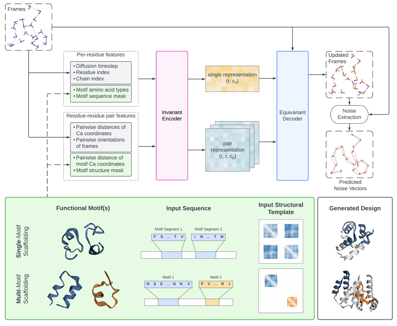
Figure : Genie 2 architecture (top), which extends Genie to enable scaffolding on (multiple) motifs. It consists of an SE(3)-invariant encoder that transforms input features into single residue and pair residue-residue representations, and an SE(3)-equivariant decoder that updates frames based on single representations, pair representations, and input reference frames. Example inputs to the model for single- and multi-motif scaffolding problems are shown (bottom-left green box), along with the corresponding generated designs (bottom-right box). In single motif scaffolding (top row), the motif may be contiguous or non-contiguous but all inter-residue positions and orientations are defined. In multi-motif scaffolding (bottom row), inter-motif geometry is left unspecified. For input sequences, white boxes denote masked out regions corresponding to the scaffold.

The denoiser’s job is to predict what noise was added at timestep t. The predicted noise is then used in the $\mu_\theta$ formula to denoise $x_t$ to $x_{t-1}$. Genie’s denoiser has two main components:

1. SE(3) - Invariant Encoder

2. SE(3) - Equivariant Decoder

SE(3) - Invariant Encoder

Input:

• Per-residue features:
  • Diffusion timestep t
  • Residue index (position in chain)
  • Chain index (which chain, for multi-chain proteins)
  • Motif amino acid types (if doing motif scaffolding)
  • Motif sequence mask (which positions are part of motifs)

• Residue-residue pair features:
  • Pairwise distances of C$\alpha$ coordinates
  • Pairwise orientations of frames (how frames are rotated relative to each other)
  • Pairwise distances of motif C$\alpha$ coordinates
  • Motif structure mask

Output:

• Single representation: Features for each individual residue

• Pair representation: Features for each pair of residues

The encoder processes these features in a way that’s SE(3)-invariant which means that the output does not change if you rotate/translate the entire protein. Looking at the input features above, we can see that none of them should change if you rotate or translate the entire protein. Hence, the encoder must have the same understanding regardless of absolute orientation. The encoder is trying to learn “what patterns exist in this structure?” These patterns can be “these residues form a helix”, “this region is a loop” or “these positions interact strongly” and none of these patterns depend on absolute orientation. The output representations capture relationships between residues in a coordinate-free way.

SE(3) - Equivariant Decoder

Input:

• Single representations from encoder

• Pair representations from encoder

• Input reference frames $F(x_t)$

Output:

• SE(3)-equivariant frame predictions $F'(x_t)$

The decoder uses Invariant Point Attention (IPA) as used in AlphaFold2. In a nutshell, IPA does the following in an SE(3)-equivariant way:

1. Takes single and pair representations

2. Uses attention mechanisms to mix information between residues

3. Updates the single representations based on geometric relationships

Equivariant means that the decoder updates frames such that if you rotate/translate the input, the output rotates/translates in the same way. The updated single representations are used to update the reference frames from $F(x_t)$ (noisy) to $F'(x_t)$ (prediction of less noisy). Each frame has a translation component $t \in \R^3$ and a rotation component $R \in SO(3)$ (Special Orthogonal, it is like a 3x3 rotation matrix).

Questions about Encoder-Decoder

1. Why do we need an Encoder-Decoder architecture? Why not just process the raw features directly?

   The inputs we currently have are raw features like timestep, residue indices, distances etc which are low-level, sparse and local information. In order to update the frames, we need a rich, contextual understanding of the entire protein structure. We need to know what the global patterns are like “This region forms a helix”, we’d need to know about the long-range interactions “Residue 10 affects residue 50”, we’d need to know the structural constraints “These motifs need to be connected”.

   The encoder transforms inputs into information-rich intermediate representations. They act like compressed knowledge and they are no longer just the raw input features but rather a learned understanding of what those features mean structurally. The decoder uses the rich understanding to make informed geometric predictions.

   Without the encoder, if we fed raw features directly to the decoder, there would be several problems:

   • Having to learn too much simultaneously: Learning to extract patterns from raw features, learning geometric reasoning, learning denoising strategy
   • Poor information flow since there is no global context about overall structure and cannot reason about long-range interactions
   • Inefficiency: Raw features are high-dimensional but not informative and the network wastes capacity processing irrelevant details

   With encoder, the decoder works with a rich context.

2. Why should the encoder be SE(3)-invariant and why should the decoder be SE(3)-equivariant?

   The encoder computes features describing each residue and features describing relationships between residues. These representations must not change if we translate/rotate the entire protein. The encoder must output the same understanding regardless of absolute orientation.

   The decoder computes the actual 3D positions and orientations. If the entire protein is translated/rotated, then these predictions must transform in the same way. If the output did not rotate according to the input, then we’d get physically nonsensical results.

   If the encoder was not invariant, then the network would treat the same structure differently just because of rotation. As a consequence, the network learns the same structure patterns multiple times (once per orientation). This would lead to poor generalization and the network would need to see every structure in every possible orientation during training.

   If the decoder was not equivariant, the geometric predictions would not be consistent with input orientation and we’d get physically invalid outputs.

   Encoder asks: “What is this?” (invariant)

   Decoder asks: “Where should this be?” (equivariant)

   Also, encoder computations are cheap since it is just processing scalar features whereas decoder computations are expensive since it processes geometric feartures and it uses specialized operations like IPA and also has to maintain SE(3) equivariance constraints. The separation makes the architecture more efficient.

3. Why calculate Pair representations if it seems like only Single representations are used to update frames?

   Pair representations don’t directly update frames but they indirectly influence the frame updates by modulating the IPA mechanism. Pair representations modulate the communication between residues.

Noise Computation

In the forward diffusion process, Genie only adds noise to coordinates and not to rotations (design choice). Rotations are computed from the local geometry of the backbone i.e. derived from positions, they are not independent variables that get noised separately. Models like FrameDiff and FrameFlow diffuse on SE(3) space directly (position and rotation). However, Genie diffuses only on positions and rotations follow from positions.

Input frames: $F(x_t) = [(t_1, R_1), (t_2, R_2), ...]$. Both $t$ and $R$ are noisy since they both come from noisy positions.

Updated frames: $F'(x_t) = [(t'_1, R'_1), (t'_1, R'_1), ...]$. Network predicts better positions $t'$. Rotations $R'$ are recomputed from the updated positions.

Noise $\epsilon_\theta = t' - t$, which is just the position displacement. We do not extract rotation noise because rotations weren’t independently noised, the rotation denoising happens implicitly when you denoise the positions.

Methods

Genie 2 extends Genie architecture and training procedure to enable motif scaffolding.

Motif representation for conditional generation Genie’s architecture naturally permits integration of conditional sequence and structure information into the diffusion process. We do so by encoding the residues of each motif as one-hot vectors and concatenating these encodings to the single residue features. We encode the structure of each motif using the pairwise distance matrix of its Cα atoms. This representation is SE(3)-invariant as it does not encode the absolute position and orientation of the motif(s), and is unlike the motif conditioning procedures of other methods (e.g., RFDiffusion and FrameFlow), which fix motif coordinates and are thus sensitive to initial placement(s).

Our approach sidesteps a challenge in multi-motif scaffolding, where the design objective leaves the relative positions and orientations of motifs unspecified. By representing motif structures using pairwise distance matrices that specify intra-motif but not inter-motif distances, Genie 2 learns to satisfy the constraints of each motif while generating self-consistent configurations of inter-motif geometries. Figure 1 illustrates the types of (multi-)motif templates that can be specified. Note that even in single motif scaffolding, a motif may be non-contiguous by comprising multiple segments. What differentiates single and multi-motif scaffolding is that inter-segment geometric relationships are specified while inter-motif relationships are not. Genie 2’s formulation does require specifying sequence length separations between motifs, either by fixing them or sampling from a distribution.

A one-hot vector represents a categorical variable (like amino acid type) as a binary vector with exactly one “1” and the rest “0s”. For amino acid it would look like:

$[0, 0, 0, 0, 0, 0, 0, 1, 0, 0, 0, 0, 0, 0, 0, 0, 0, 0, 0, 0]$

Each amino acid gets a unique 20-dimensional vector with exactly one 1.

For each residue position, the encoder processes “per-residue features” like Diffusion timestep (t), residue index etc. (refer above) which are all numerical features for each residue position to generate Single Residue features. For a scaffold position, the motif encoding would be 20-dimensional with all 0s and for a motif position, the motif encoding would be 20-dimensional with one 1 corresponding to the amino acid. For a protein with N residues, let’s say for each residue the base features are in a b-dimensional vector. The motif encoding vector is 20-dimensional. So after concatenation, the the final vector would be (b+20)-dimensional vector. The final shape would be (N, b+20). Hence, the concatenation tells the network which positions are motif and which are scaffold and what amino acid type each motif position is. The structure of each motif is encoded using the pairwise distance matrix of its C$\alpha$ atoms.

Training

Genie 2 is trained to do motif scaffolding by creating synthetic training tasks from real protein structures. The idea is to take a complete protein, randomly extract part of it as a “motif” and then train the model to regenerate the rest (scaffold). Genie 2 is trained in a purely conditional manner meaning that every training example has a motif constraint (no training on unconditional generation whatsoever). The training task is basically:

1. Sample a real protein structure from the dataset (”ground truth”)

2. Randomly designate part of it as a motif

3. Train model to generate the scaffold around that motif

Random Sampling Parameters

$N_s \sim U(1, 4)$ - Number of segments

The motif can have 1-4 non-contiguous segments (uniform distribution). Examples:

• $N_s = 1$ - Single continuous segment (say residues 20-30)

• $N_s = 3$ - Three segments (say residues 10-15, 40-45, 80-90)

Real functional motifs are often non-contiguous so we need to account for multiple segments.

$N_r \sim U[\lfloor 0.05N\rfloor, \lceil 0.5N \rceil]$ - Number of residues

$N$ - Total protein length

The motif contains between 5% and 50% of the protein’s residues.

Algorithm

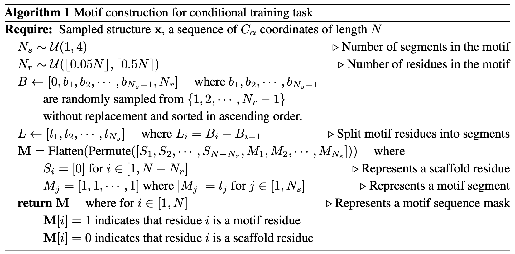
Let the total protein length $N = 200.$

B is the boundary array that defines where each segment starts in the sequence. It divides the $N_r$ motif residues into $N_s$ segments. Example: $N_r$ = 45 residues to split into $N_s$ = 3 segments. Sample 2 ($(N_s - 1 = 2)$ boundaries: $b_1 = 15$ and $b_2 = 32$. Hence, $B = [0, 15, 32, 45].$ This creates 3 segments but these are just abstract indices, we haven’t placed them in the protein yet.

L captures the segment lengths.
$l_1 = B_1 - B_0 = 15-0 = 15, \space l_2 = B_2 - B_1 = 32-15 = 17, \space l_3 = B_3 - B_2 = 45-32 = 13$
$L = [15, 17, 13]$

$M$ is the binary mask that indicates which residues are motif and which are scaffold. There are $S = N - N_r = 200 - 45 = 155$ scaffold positions.

Permute randomly shuffles the scaffold zeros and motif segments. Before flatten and after permute, the list would look like:

$[[0], [1,1,...,1](17 \space ones), [0], ..., [0], [1,1,...,1](15 \space ones),...]$After flatten, it would look like:

$[0,1,1,...,1(17 \space ones), 0, ..., 0, 1,1,...,1(15 \space ones),...]$

It was observed that training only on motif scaffolding tasks works better than mixing with unconditional generation. Every single training example has a motif which forces the model to learn constraint handling.

Genie 2’s performance on multi-motif scaffolding thus represents out-of-distribution generative generalization.

Genie 2 is trained on single motif with known inter-segment distances but during testing we can get multiple motifs with unknown inter-motif distances. Hence, the model must generalize to a harder problem it never saw during training.

Data Augmentation

As AFDB is highly structurally redundant, we use a subsampled version [5] that applies FoldSeek [38] to cluster entries based on structural similarity. We start with all cluster representatives from the FoldSeek-clustered database and then filter them using a pLDDT threshold of >80, to enrich for highly confident predictions, and a maximum sequence length of 256.

AFDB = AlphaFold Database

pLDDT (predicted Local Distance Difference Test) - AlphaFold’s confidence score for each residue. Scale: 0-100, 80 = high confidence.

The problem is the AFDB contains many predicted protein structures that are very similar to each other like same protein from different organisms or proteins from the same family with minor variations etc. This would be bad for training as the model can overfit or the model might not learn diverse structural patterns efficiently.

FoldSeek is a tool that clusters proteins based on their 3D structural similarity (not sequence similarity).

Loss function

The goal is to train the model to predict the noise that was added during the forward diffusion process.

$L(\theta) = \mathbb{E}_{t,x_0,\epsilon}\big[ \frac{1}{N} \sum_{i=1}^{N} \left | \left | \epsilon_t^i - \epsilon_\theta^i(F(x_t), t)\right | \right |^2 \big] \newline \newline = \mathbb{E}_{t,x_0,\epsilon}\big[ \frac{1}{|\mathbb{M}| + |\mathbb{S}|} \left ( \sum_{i \in \mathbb{M}} \left | \left | \epsilon_t^i - \epsilon_\theta^i(F(x_t), t)\right | \right |^2 + \sum_{i \in \mathbb{S}} \left | \left | \epsilon_t^i - \epsilon_\theta^i(F(x_t), t)\right | \right |^2 \right ) \big]$

$\mathbb{M}$ and $\mathbb{S}$ are the set of motif and scaffold residue indices respectively.

What this means is for each training step, sample a protein, sample timestep and sample noise, add noise, model predicts the added noise and compute the loss as the average squared difference across all residues.

Under this construction, motifs are enforced as a soft constraint, ensuring that the model is responsive to motif specifications while also designing the protein as a whole.

It is not a hard constraint because the loss is not computed over the scaffold positions only, rather the loss is computed on all positions. If we only had motif term, the model only learns to denoise motif positions ignoring the scaffold leading to bad scaffolds. If we only had scaffold term, the model only learns scaffold and might not respect motif constraints. With both terms, the model learns to denoise motif positions while maintaining their structure and generate a scaffold that is compatible with motif.

Unconditional Protein Generation Analysis

Important Concepts

TM-score

• Template Modeling score

• Measures the structural similarity between two protein structures ranging from 0 to 1

• TM-score > 0.6 indicates high confidence of structural similarity

• TM-score is length-independent and is more sensitive to global topology. It is better than RMSD (root mean square deviation) because RMSD measures average distance between corresponding atoms in Angstroms but longer proteins have higher RMSD even if structurally similar. TM-score normalizes this.

• Intuitively it helps ask “do these proteins have the same overall architectural fold” rather than “are all atoms in exactly the same positions?”

TMAlign

• An algorithm that aligns two protein structures by finding the optimal superposition and computes their TM-score.

• Alignment matters because proteins can have the same structure but different positions/orientations in 3D space.

• TMAlign rotates and translates them to find the best overlap before measuring similarity.

Hierarchical Clustering with Single Linkage

• Hierarchical clustering is a bottom-up grouping algorithm. Initially, each structure is its own cluster. Until a similarity threshold is reached, two closest clusters are merged.

• Single linkage - “distance” (not exactly like distance) between two clusters is the minimum distance between any pair of points across clusters. For example:

  Cluster A: {structure 1, structure 2}

  Cluster B: {structure 3, structure 4}

  Distance(A, B) = min(TM(s1, s3), TM(s1, s4), TM(s2, s3), TM(s2, s4))

• Suppose the TM-score threshold is 0.6, then we can stop merging when all remaining cluster pairs have TM-score $\le 0.6$. Each final cluster contains structurally similar proteins and different clusters are structurally distinct.

Four Evaluation Metrics

Designability

• Tries to answer “Can this generated structure actually be made by a real protein sequence?”

• Pipeline -
  • Step 1: Generated Structure
  • Step 2: Inverse folding through ProteinMPNN gives 8 plausible sequences for the structure
  • Step 3: Each of the 8 sequences is folded into predicted structures using ESMFold
  • Step 4: Compare the predicted structures with the original generated structure.

• in silico - by means of computer modeling/simulation

• Designability criteria that must be satisfied:
  • scRMSD $\le 2\r{A}$ - Self-consistency RMSD. The closest predicted structure is within $2\r{A}$ of the original.
  • ESMFold’s confidence score i.e mean pLDDT must be $\ge 70.$

• For a set of $N$ structures, designability is the number of designable structures among them.

• This test is important because a structure might look chemically valid but may be impossible to realize with any amino acid sequence so it’s important to check if there is a sequence that actually folds into this structure.

• Potential problem - Mode collapse. Suppose there is a model that always generates the same valid protein structure, in this case the designability is 100% but it is useless because there is no diversity.

Diversity

• Tries to answer “How many structurally distinct, viable proteins can the model generate?”

• Algorithm -
  • Filter to only designable structures since non-designable structures are unrealizable
  • Compute all pairwise TM-scores using TMAlign
  • Hierarchical clustering with single linkage with a threshold of 0.6
  • Count the number of distinct clusters

• Diversity is then computed as the number of distinct clusters from the total number of structures generated.

• TM-score threshold of 0.6 is a conventional cutoff where structures are considered to have different folds. A stricter threshold of 0.8 would split similar structures and a looser threshold of 0.4 would group distinct folds together.

• Diversity enforces designability through step 1, so it is a stronger metric than designability alone.

• Diversity decreases as you generate more samples (more likely to hit existing clusters) which is why comparisons require fixed sample sizes.

F1 score

• Tries to answer “What is the balanced performance on both designability and diversity?”

• Harmonic mean heavily penalizes imbalance

• The $\beta$ parameter controls relative importance. $\beta > 1$ favors diversity and $\beta < 1$ favors designability. Genie 2 uses $\beta = 1$.

• The F1 score matters because it forces models to balance two competing objectives.

Novelty

• Tries to answer “Are we generating new protein folds or just recreating known ones?”

• PDB and AFDB are the two reference datasets

• Algorithm -
  • For each designable structure, compute TM-scores to ALL structures in reference dataset
  • Novel if TM-score $\le$ 0.5 to all reference structures
  • Cluster the novel structures (threshold 0.6)
  • Count distinct novel clusters

• Novelty is the number of distinct novel clusters from the total number of structures generated.

• TM-score below 0.5 indicates different folds, so novel structures have new folds not seen in the reference dataset.

In-distribution performance analysis

• Secondary structures - alpha helices (spiral structures), beta strands/sheets (extended, pleated structures), loops/coils (flexible connecting regions)

• It was found that models generate proteins biased toward alpha helices compared to AFDB which shows more uniform distribution

• Possible reasons for helix bias:
  • AFDB has many helical structures so models learn this distribution
  • Beta sheets are harder to generate because helices involve local interactions whereas sheets involve long-range interactions
  • Low temperature is used to get better quality results which pushes the model toward high-probability (helical) structures rather than exploring the full distribution

• Structures are generated at two temperatures. At lower temperatures the the model picks the highest probability structures whereas at normal temperature, $\gamma = 1$, Genie2’s distribution matches AFDB much better.

• It was found that the training data (AFDB structures) has lower designability than experimental structures (PDB structures). However, with relaxed criteria $(scTM \ge 0.5, pLDDT \ge 70)$, AFDB structures are much more designable.

• This tells us that the AlphaFold predictions are globally reliable (overall fold is correct $scTM \ge 0.5$) but they are locally inaccurate (imprecise atomic details, $scRMSD \gt$ 2$\r{A}$).

• ProteinMPNN was trained on high-quality PDB structures, so when given an AFDB structure with imprecise atomic details, it generates sequences that fold correctly in general but don’t match the precise atomic positions in the AFDB structure.

• Hence, a low temperature helps since it biases toward high-confidence structures which might implicitly push toward more PDB-like structures yielding better designability scores.

• Temperature tradeoff - $\gamma=1$ gives structures matching the training AFDB distribution whereas a $\gamma \lt 1$ gives structures ProteinMPNN can design but represents a biased distribution.

Length-based performance analysis

• Short proteins are a small design space, yet Genie2 achieves a high diversity here.

• Tougher to generate larger proteins due to their increased complexity.

• As sequence length increases, designability decreases and so does diversity as it depends on the former.

• In principle, larger protein lengths can allow pore possible folds leading to higher diversity but they are harder to generate.

• Genie2 has extremely good generalization since it can perform well for lengths 2x the training length.

Motif Scaffolding

Success is measured by unique structures (important practically) not just success rate since it is possible to achieve a high success rate by repeatedly generating only one or few successful designs (mode collapse).

Biological terms I encountered:

Epitope

• A small, specific 3D region on a protein that can be recognized and bound by an antibody or immune cell receptor.

• Analogy - epitope is the lock shape on the surface of a protein, antibody is the key that fits this specific shape. When they match, the antibody binds to the epitope.

• For example, a virus surface protein can have multiple epitopes. Different antibodies recognize different epitopes and targeting multiple epitopes leads to a stronger immune response making it harder for the virus to escape.

Immunogen

• A molecule (usually a protein) that triggers an immune response and produces antibodies.

• By scaffolding specific epitopes, we can design an immunogen that is more targeted by presenting only the epitopes we want an immune response against.

Binder

• A protein designed to bind (stick to) a specific target protein.

• Think of it as a custom-designed molecular velcro.

• Designing binders has therapeutic applications. For example:
  • block a harmful protein’s function (like blocking a virus from entering cells)
  • deliver drugs to specific cells (binder finds the target, carries drug)
  • modulate protein function (change how a protein works)

Heterodimer

• A complex made of two different protein subunits stuck together.

Limitations and Future Work

• Genie 2 sampling time is longer than that of other methods, requiring 1000 denoising iterations (Genie 2 takes longer time to generate structure compared to other models).

• Genie 2 uses triangular multiplicative update layers introduced in AlphaFold2. Computationally expensive with $O(N^3)$ scaling.

Questions

Might be more on the biology side

How exactly is the task for generating a scaffold for a single motif with multiple segments different from the task of multi-motif scaffolding?

What does it mean when you say “motifs are enforced as a soft constraint”? Does it mean motif can deviate slightly if it improves the overall structure? What implications can it have on the goal in hand? What if the goal involved generating a protein where there must be no changes to the motif whatsoever?